Model Predictive Control
Published:
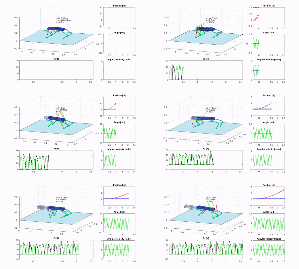
The below animation depicts a Model Predictive Control on a dynamic four-legged robot by Yanran Ding.
Over the years, the advancement in robotics and related areas has allowed robot models to have complex and non-linear dynamic equations. The application of such robots involves dynamic environments or environments which are highly inaccessible to humans. Such robot models introduced new challenges in the control strategies as typical industrial controllers such as PID controllers can fail in guaranteeing many features in these areas. These new challenges lead to extensive research to develop optimal control strategies to satisfy the needs of different applications. One such strategy developed by researchers is Model Predictive Control (MPC).

One of the first-ever applications of MPC was in chemical plants to control the transients of dynamic systems with hundreds of inputs and outputs, subject to constraint. But MPC has come a long way since then, with its application covering many fields and significant improvement in its technical capabilities.
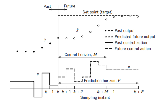
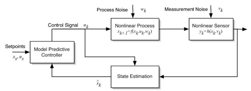
Imagine walking in a dark room; we first try to sense our surroundings, then based on that, we try to predict the best path towards our goal, and finally, we take only one step on that path and then repeat this entire cycle. MPC also works on a very similar line of reasoning. The essence of MPC is to optimize the manipulatable inputs and the forecasts of process behavior. If we have a reasonably accurate dynamic model of a system, we can use this model and current measurements to predict the future outputs of the system. We can then make the appropriate changes in the input variable based on these predictions.

At each timestep, MPC solves an open-loop optimization problem for the prediction horizon to compute control. The prediction horizon decides how far in the future should the model predict the state of the system. The sequence of control moves calculated by the model corresponding to these predictions is called the control horizon. Even though a sequence of multiple control moves is calculated at each sampling instant, only the first move is implemented on the system. This is the reason why MPC is also called receding horizon control. After this, a new sequence is calculated for the next sampling instant, after the latest measurements become available, and again only the first input move is implemented.
One obvious question that arises in mind is why we are calculating a sequence of multiple inputs if we are applying only the first input? A significant benefit of MPC arises from determining the optimal operating conditions (setpoints) and moving the process to these set points in an optimal manner based on the control calculations. By applying only the first input and recalculating the control moves based on new predictions, we ensure that all inputs are based on the optimal operating conditions, irrespective of how our system parameters are changing with time.
MPC relies on the provided model for its computations. The model selection has a significant role in the algorithm’s computational complexity, like its theoretical properties (e.g. stability). At the same time, the selected objective and imposed constraints also influence and define these properties.
Another critical benefit of MPC is its ability to handle inequality constraints. Inequality constraints were a primary motivation for the early development of MPC. Input constraints occur due to physical limitations on the system such as motors, pumps, etc.
MPC can explicitly handle constraints on both input and output because of its approach of solving open-loop optimization problems for the cost function, which can be solved easily subjected to given constraints. The nature of the optimization problem in linear MPC is a convex function, i.e. the polygon area over which optimization occurs are convex polygons. These problems are commonly referred to as Convex Quadratic Program (QP).

The optimization problem commonly used in MPC is the finite-time optimal control problem (FTOCP), i.e. the cost function is optimized for a finite horizon by imposing a terminal constraint.

Some other benefits of MPC include allowing time delays, inverse response, inherent nonlinearities (changing dynamics), and changing control objective and sensor failure because of its predictive nature.
If we think about the quadruped simulation (RF-MPC on quadruped) we saw above, we can understand why MPC is a popular choice for such systems. Designing and controlling a legged robot requires the control design to use its inherent dynamics while dealing with constraints due to hardware limitations and interactions with the environment, which are some of the significant benefits of MPC. The movement of legged robots mainly involves controlling the joint angles of the legs. The inputs given to motors present at these joints must be strictly within a specific range as any arbitrary movement of legs can lead to damage to the robot. In legged robots, multiple variables are required to be controlled, such as joint angles, CoM of the robot, the robot’s velocity, the velocity of the end effectors etc., which can be handled conveniently by MPC by designing a multi-variable cost function.
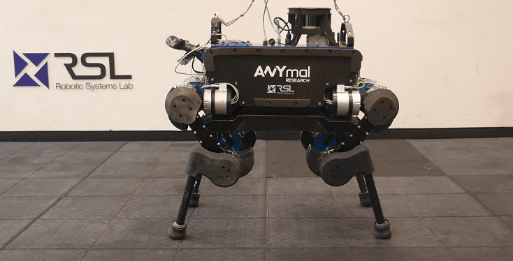
Some of the popular robots that use MPC are ANYmal by ETH Zurich, Atlas by Boston Dynamics and MIT Cheetah.
Variants of MPC
Non-Linear MPC: Nonlinear Model Predictive Control, or NMPC, is a variant of model MPC, characterized by non-linear system models. NMPC also requires the iterative solution of optimal control problems on a finite prediction horizon as in linear MPC. While these problems are convex in linear MPC, in non-linear MPC, they are not necessarily convex anymore.
Explicit MPC: Explicit MPC (eMPC) allows fast evaluation of the control law for some systems, in stark contrast to the online MPC. Explicit MPC is based on the parametric programming technique (optimization problem is solved as a function of multiple parameters). The solution to the MPC control problem formulated as an optimization problem is pre-computed offline. This offline solution, i.e. the control law, is often in the form of a piecewise affine function (PWA).
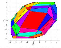
Other than these, there are many more variants of MPC coming up, such as robust MPC and Hybrid MPC, which can account for set bounded disturbance while still ensuring state constraints are met.
Given its remarkable success, MPC has been a popular subject for academic and industrial research. Significant extensions of the early MPC methodology have been developed, and theoretical analysis has provided insight into the strengths and weaknesses of MPC. There are many well-documented implementations of MPC available online one of such implementation is by Atsushi Sakai. Matlab also has an inbuilt toolbox specifically dedicated to MPC. To understand more about Model Predictive Control you can also visit the ERC handbook page.
References
- Seborg, D. E.; Mellichamp, D. A. & Edgar, T. F. (2011), Process Dynamics and Control, John Wiley & Sons. (Chapter 20th, Model Predictive Control)
- Ruchika, Neha Raghu.” Model Predictive Control: History and Development”. International Journal of Engineering Trends and Technology (IJETT)
- What is Model Predictive Control (MPC), Mitesh Agrawal, August 10, 2020
- Prof. S. Boyd, EE364b, Stanford University
- EE392m - Spring 2005, Gorinevsky, Stanford University
- Y. Ding, A. Pandala and H. -W. Park, “Real-time Model Predictive Control for Versatile Dynamic Motions in Quadrupedal Robots,” 2019 International Conference on Robotics and Automation (ICRA)
- Linear Model Predictive Control, Autonomous Robots Lab
